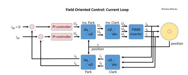
Figure: Field-Oriented Control — Current Loop Block Diagram
This guide explains how a PMSM motor is controlled — from the basic idea of torque and flux, through the mathematical transforms, all the way to real-world sensor choices. Written in plain language, with block diagrams, worked examples, and real-world analogies throughout. |
1. What is a PMSM Motor?
PMSM — Permanent Magnet Synchronous Motor
A PMSM is an AC electric motor that uses permanent magnets embedded in or on the rotor to create a fixed magnetic field. The stator carries three-phase windings that produce a rotating magnetic field. The rotor ‘locks on’ to this rotating field and spins in perfect synchronism with it — that is what ‘synchronous’ means. PMSMs are widely used in EVs, robotics, automation, and renewable energy systems due to their high efficiency, compact size, and superior dynamic performance compared to induction and brushed DC motors.
A PMSM works by synchronising the stator and rotor magnetic fields. The stator carries a three-phase winding powered by an AC supply, producing a rotating magnetic field (RMF). The rotor’s permanent magnets lock onto this rotating field and rotate at exactly the same speed. Unlike induction motors, which rely on rotor current to generate torque, PMSMs use permanent magnets to establish the rotor field, leading to higher efficiency and lower losses. Removing rotor windings also boosts reliability and reduces heat.
🧲 ANALOGY — The Spinning Compass Needle Imagine a compass needle (the rotor’s permanent magnet) inside a box with a slowly rotating magnetic field around it (the stator). The compass needle locks onto the rotating field and spins with it perfectly — never slipping. If you spin the field faster, the needle follows. This perfect lock-step is what ‘synchronous’ means. ➤ In motor terms: The PMSM rotor flux is fixed by the permanent magnets. The control system generates a rotating stator field by varying the three-phase currents (Amperes). The rotor chases this field. The control goal is always to keep the stator current vector exactly 90° ahead of the rotor flux — this angle maximises the torque (Nm) produced. |
1.1 SPMSM vs IPMSM — Two Designs
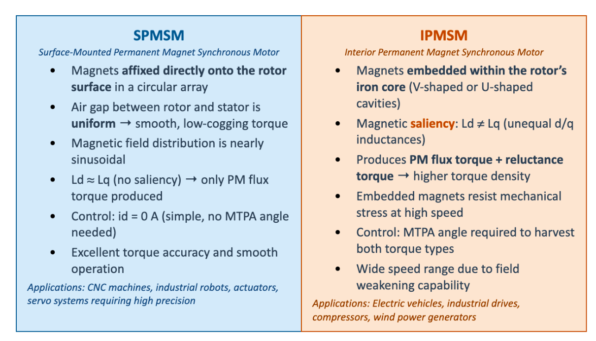
PMSMs are not all the same — their rotor design fundamentally influences performance. Two main types exist, differing in structure, control complexity, and ideal application:
1.2 Motor Cross-Section Diagrams
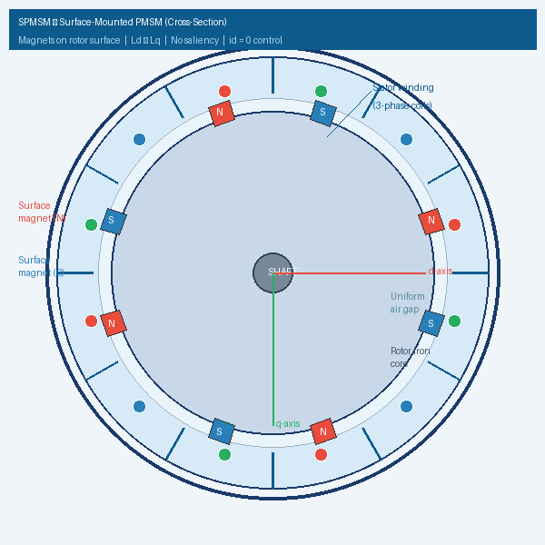
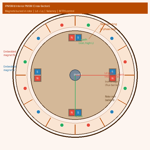
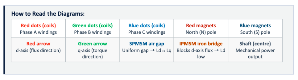
The diagrams below show a simplified cross-section of each motor type, viewed from the end of the shaft. Key features — stator slots, rotor, magnet positions, d-axis, and q-axis — are all labelled.
1.3 Key Structural Differences
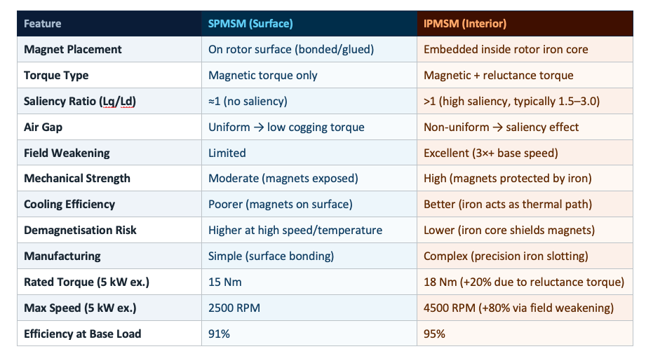
The structural difference between SPMSM and IPMSM forms the foundation for all their contrasting characteristics. This table uses real data:
1.4 Efficiency Comparison by Speed (Real Data)
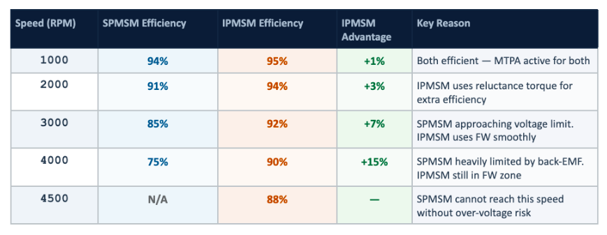
The efficiency difference between SPMSM and IPMSM becomes more pronounced at higher speeds. The IPMSM’s ability to use field weakening prevents back-EMF saturation, maintaining high efficiency at speeds where the SPMSM loses significantly:
Source note: |
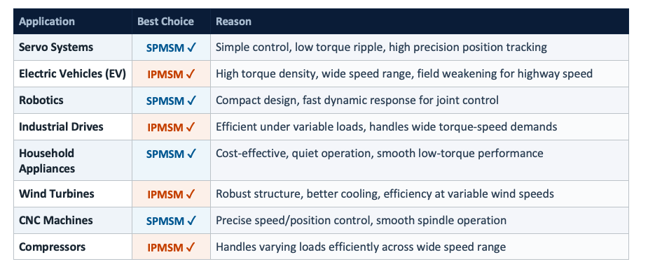
1.5 Application Suitability Guide
Each motor type has distinct advantages based on application priorities. Use this table as a quick selection guide:
1.6 Case Study: EV Traction Motor — 100 kW System
To illustrate the real-world performance gap, consider a 100 kW electric traction system tested with both SPMSM and IPMSM configurations under identical voltage and current limits. This data explains why major EV manufacturers — including Tesla and Toyota — use IPMSM in their traction drives:
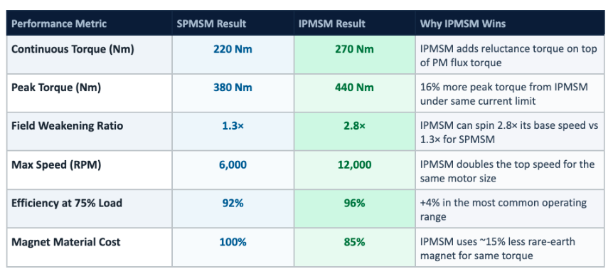
🚗 | Why Tesla and Toyota use IPMSM The 100 kW case study makes it clear: IPMSM delivers 23% more peak torque, 2× the top speed, 4% better efficiency, and 15% less magnet cost for the same power rating. For an EV where range, acceleration, and top speed are all critical, IPMSM is the only practical choice for the traction motor. |
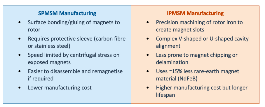
1.7 Manufacturing, Maintenance & Future Trends
🔬 | Future Trends Engineers are now developing hybrid PMSMs combining surface and interior magnet arrangements — harvesting both high low-speed torque and efficient field weakening. Other advances: segmented magnets (reduce eddy current losses), high-temperature alloys (SmCo / NdFeB with dysprosium), AI-driven real-time current vector optimisation, and additive manufacturing to reduce rotor assembly complexity. |
2. How Does a PMSM Produce Torque?
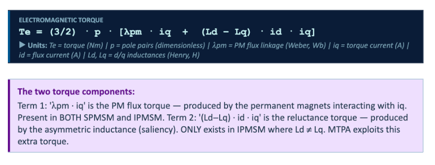
Torque (measured in Newton-metres, Nm) is produced by the electromagnetic interaction between the stator’s rotating magnetic field and the rotor’s permanent magnets. The stator’s three-phase windings carry currents that create a rotating magnetic flux vector. The rotor magnets try to align with this vector — and in doing so, they drag the rotor round.
The key insight is: the torque is maximised when the stator current vector is kept exactly 90° ahead of the rotor flux vector. This is exactly what FOC (Field-Oriented Control) achieves — it continuously adjusts the current vector angle to maintain this 90° relationship, regardless of speed.
3. Understanding id and iq — The Two Control Levers
The clever heart of PMSM control is that engineers convert the three time-varying AC phase currents (ia, ib, ic) into just two constant DC values: id and iq. In steady state, these are DC values that PI controllers can regulate precisely.
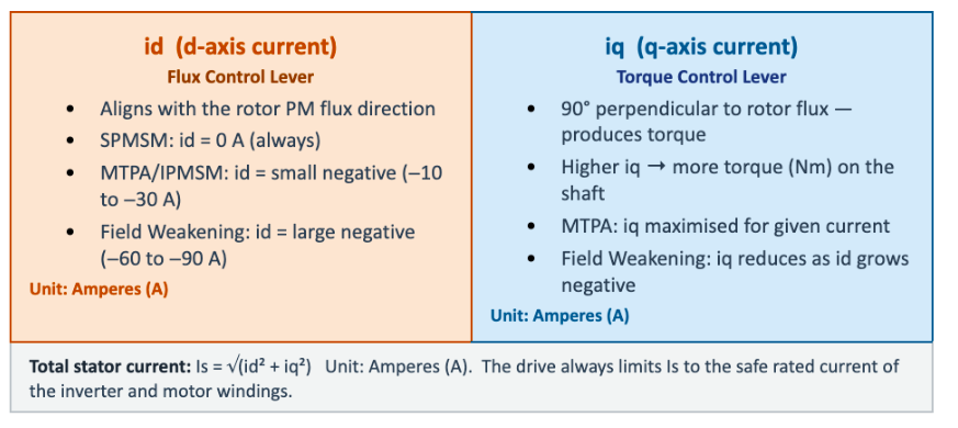
💡 | Why does this matter? As long as you control id and iq (two DC numbers in Amperes), you fully control the motor’s flux and torque. This is far simpler than trying to regulate three sinusoidal AC currents directly. The Clarke and Park transforms make this conversion possible — and it’s the foundation of all modern high-performance motor control. |
4. Field-Oriented Control (FOC) — The Core Algorithm
What is FOC?
Field-Oriented Control (FOC), also called vector control, is a method of controlling a PMSM that keeps the stator current vector precisely aligned for maximum torque production. It does this by decomposing the stator current into two DC components (id and iq), controlling each with a separate PI controller, then transforming the resulting voltage commands back to three-phase AC to drive the inverter. The result is extremely fast, precise, and efficient torque control — the same technique used in every modern EV motor drive.
4.1 FOC Current Loop — Block Diagram
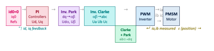
The diagram below shows the complete FOC current loop. The upper path (pink → PI → Inverse Park → Inverse Clarke → PWM) is the forward command path. The lower path (Clarke → Park → back to PI) is the measurement feedback path. Rotor position ε feeds both the Park and Inverse Park blocks.
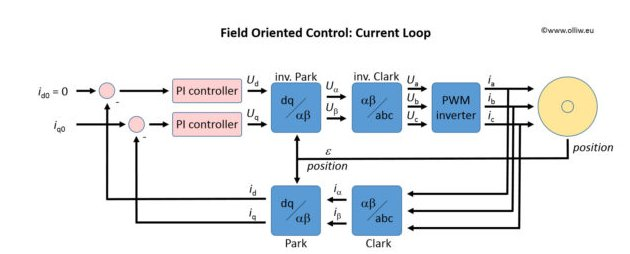
Figure: FOC Current Loop — Reference Diagram (source: www.olliw.eu)
The same loop redrawn as a block diagram with all signal labels:
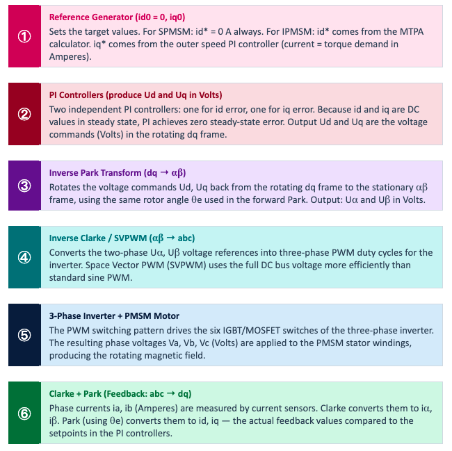
4.2 What Each Block Does
5. Clarke Transform (abc → αβ)
What does the Clarke Transform do? The Clarke Transform converts the three phase currents (ia, ib, ic — all in Amperes) into just two orthogonal currents (iα and iβ — also Amperes) in a two-dimensional stationary frame. It is a pure mathematical simplification — no rotation is applied yet. The key benefit: a 3-variable problem becomes a 2-variable problem without losing any information (since ia+ib+ic = 0 for a balanced three-phase system). |
5.1 Clarke Transform Block Diagram
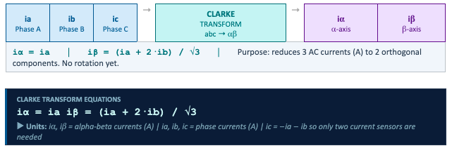
🗺️ ANALOGY — Three Friends Pointing to One Location Imagine three friends standing in a triangle, each pointing a compass in a direction 120° apart from the others, all describing the same location. The Clarke transform is like converting their three separate compass readings into one simple (x, y) coordinate — the same information, but far easier to use. You only need to track two numbers instead of three. ➤ In motor terms: The three-phase currents ia, ib, ic each differ by 120°. Clarke transforms them into iα (horizontal) and iβ (vertical) components in a stationary 2D plane. Same information, fewer variables. No rotation yet — both the abc and αβ frames are stationary. |
6. Park Transform (αβ → dq)
What does the Park Transform do? The Park Transform rotates the stationary αβ frame by the rotor’s electrical angle θe (in degrees or radians), aligning it with the rotor’s magnetic flux vector. After this rotation, iα and iβ (which were still sinusoidal AC values) become id and iq, which are DC constants in steady state. DC values are what PI controllers need to achieve zero steady-state error. |
6.1 Park Transform Block Diagram
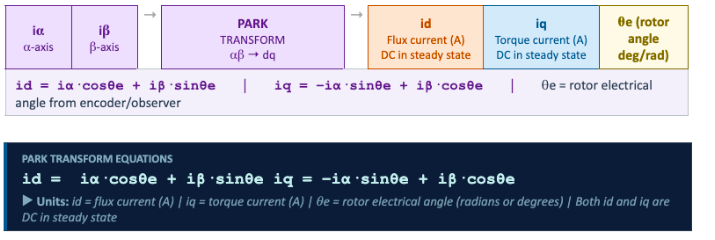
⚠️ | Why θe is critical The rotor angle θe is the key input to both the Park and Inverse Park transforms. If θe is wrong by even 5°, the id and iq values are contaminated — you lose decoupling, and torque accuracy suffers. This is why the quality of the position sensor (or the accuracy of the sensorless observer) directly determines how well the motor performs. |
🎪 ANALOGY — Riding the Merry-Go-Round Stand on the ground watching a merry-go-round: the horses appear to move continuously up and down (like AC). Now jump on and ride with it at the same speed — suddenly the horses look stationary (like DC). The Park transform is like jumping onto the rotating rotor frame. Once you rotate with the rotor at angle θe, the currents stop oscillating and become constant DC values. ➤ In motor terms: After the Park transform, id and iq are DC values that PI controllers can hold to precise setpoints with zero steady-state error. This is the fundamental reason FOC works so well: it turns a difficult AC control problem into a simple DC control problem. |
7. SVPWM — Space Vector Pulse Width Modulation
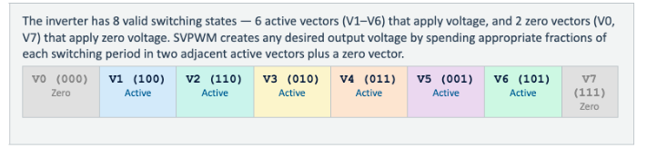
What is SVPWM?Space Vector PWM (SVPWM) is the technique used to convert the two-phase voltage references (Vα*, Vβ* in Volts) into the three PWM duty cycles (Sa, Sb, Sc as percentages) that control the six switches of the three-phase inverter. Compared to sinusoidal PWM, SVPWM uses the DC bus voltage (Volts) about 15% more efficiently, produces lower harmonic distortion in the motor current, and is easier to implement digitally on a DSP or microcontroller. |
7.1 SVPWM Block Diagram

7.2 The Eight Switching Vectors
8. Complete FOC Architecture
The full FOC control system has multiple nested feedback loops. The outer speed loop (bandwidth ~100 Hz) commands the inner current loop (bandwidth ~1 kHz). The current loop runs the Clarke, Park, PI, Inverse Park, and SVPWM pipeline every PWM switching cycle (typically every 50–100 µs).
8.1 Full Cascaded Control Loop

Loop bandwidths: Torque/current loop: bandwidth ~1000 Hz (1 kHz) — fastest loop, runs every PWM period. Speed loop: bandwidth ~100 Hz — 10× slower than current loop to prevent interaction. Position loop (if used): bandwidth ~10 Hz — 10× slower than speed loop. Rule: each outer loop must be at least 5–10× slower than its inner loop. |
9. Rotor Position Sensing — Sensored vs Sensorless
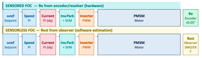
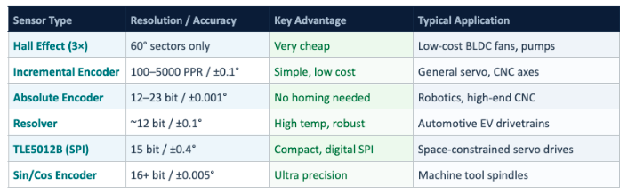
The rotor angle θe is needed by both the Park transform (feedback path) and the Inverse Park transform (forward path). How this angle is obtained defines whether the drive is sensored (measured by hardware) or sensorless (estimated by software).
9.1 Sensored vs Sensorless — Side-by-Side Block Diagrams
9.2 Position Sensor Types
9.3 Sensorless Methods
Sensorless drives estimate θe by running a mathematical model of the motor in real time. The observer uses measured phase currents and estimated or measured voltages to infer rotor position without any mechanical sensor:
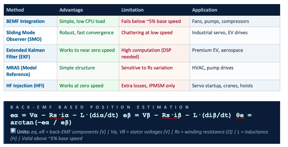
⚠️ | The Zero-Speed Problem Back-EMF = 0 at standstill (no rotation, no induced voltage). Pure BEMF sensorless methods cannot determine θe at zero speed. Solutions: (1) Initial alignment pulse — briefly force the rotor to a known position before starting. (2) High Frequency Injection (HFI) — inject a small high-frequency signal and detect position from the IPMSM’s saliency response (Ld ≠ Lq). HFI works at zero speed but only for IPMSM. |
10. MTPA and Field Weakening
These two strategies define how the motor is driven across its full speed range:
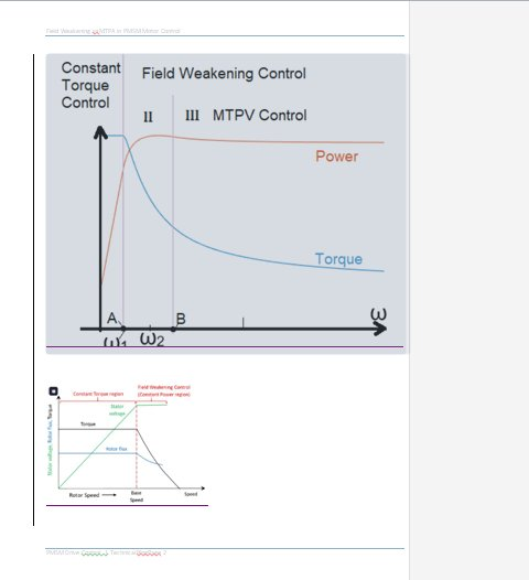
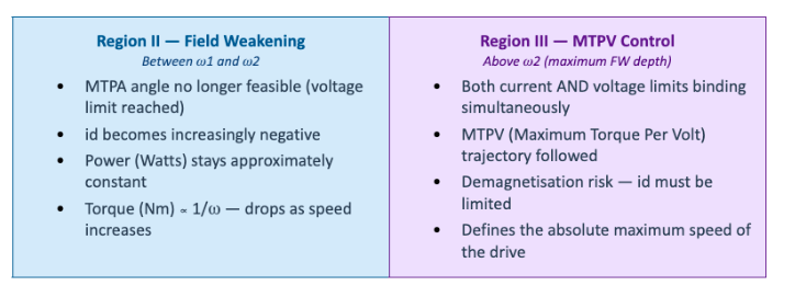
Figure: PMSM Torque-Speed Envelope — Constant Torque (MTPA) and Field Weakening regions with ω1 (base speed) and ω2 marked
10.1 MTPA — Maximum Torque Per Ampere (below ωbase)
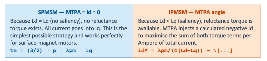
What is MTPA? MTPA finds the optimal combination of id and iq (both in Amperes) that produces the required torque (Nm) while drawing the minimum total current Is (Amperes). For SPMSM this is simply id = 0 A. For IPMSM, MTPA tilts the current vector slightly negative in the d-axis to also generate reluctance torque — producing more total Nm per Ampere than the pure iq-only approach. |
10.2 Field Weakening — Above ωbase
What is Field Weakening? As the motor spins faster, the back-EMF it generates grows. Eventually it reaches the inverter’s DC bus voltage limit (Vmax in Volts). At this ‘base speed’ (ω1), normal control is no longer possible. Field Weakening injects negative id current (Amperes) to partially cancel the permanent magnet flux, reducing back-EMF below Vmax. This allows the motor to spin faster — but torque (Nm) decreases because some current capacity is now used for flux control instead of torque production. |
Summary
What We Covered
|